Working with cortical streamlines

In this example we walk through various methods that use the Allen streamlines. Streamlines are the paths that connect the surface of the isocortex to the lower white matter surface while following the curvature of these surfaces.

Depth lookup

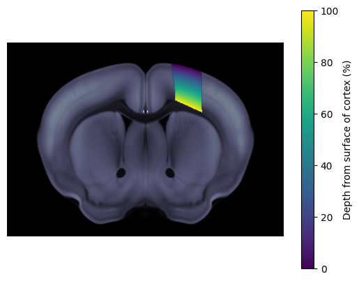
We can use the streamlines to find the depth of coordinates in 3D space relative to the surface of the cortex. Note as the streamlines are only defined in the cortex so this lookup will only work for coordinates that lie within the Isocortex of the Allen atlas volume. In this example we obtain the depths in percentage, where 0 % indicates the surface of the isocortex and 100 % the white matter boundary.

from iblatlas.streamlines.utils import xyz_to_depth
from iblatlas.atlas import AllenAtlas
import numpy as np
import matplotlib.pyplot as plt

ba = AllenAtlas()
# In this example we are going to get out the coordinates of the voxels that lie within the region MOp
region_id = ba.regions.acronym2index('MOp')[1][0][0]
# MOp is in the beryl mapping so we map our label volume to this mapping
ba.label = ba.regions.mappings['Beryl-lr'][ba.label]
# These are the indices in the volume, order is AP, ML, DV
ixyz = np.where(ba.label == region_id)
# Convert these to xyz coordinates relative to bregma in order ML, AP, DV
xyz = ba.bc.i2xyz(np.c_[ixyz[1], ixyz[0], ixyz[2]])

depth_per = xyz_to_depth(xyz) * 100

# We can assign a volume
depth_per_vol = np.full(ba.image.shape, np.nan)
depth_per_vol[ixyz[0], ixyz[1], ixyz[2]] = depth_per

fig, ax = plt.subplots()
ba.plot_cslice(620/1e6, volume='image', ax=ax)
ba.plot_cslice(620/1e6, volume='volume', region_values=depth_per_vol, ax=ax, cmap='viridis', vmin=0, vmax=100)
ax.set_axis_off()
cbar = fig.colorbar(ax.get_images()[1], ax=ax)
cbar.set_label('Depth from surface of cortex (%)')

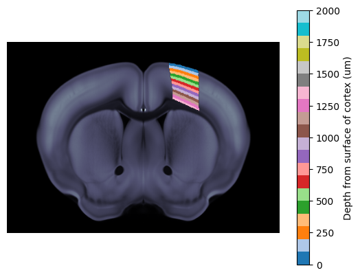
We can also do this look up in um relative to the surface of the cortex.

depth_um = xyz_to_depth(xyz, per=False)

# We can assign a volume
depth_um_vol = np.full(ba.image.shape, np.nan)
depth_um_vol[ixyz[0], ixyz[1], ixyz[2]] = depth_um

fig, ax = plt.subplots()
ba.plot_cslice(620/1e6, volume='image', ax=ax)
ba.plot_cslice(620/1e6, volume='volume', region_values=depth_um_vol, ax=ax, cmap='tab20', vmin=0, vmax=2000)
ax.set_axis_off()
cbar = fig.colorbar(ax.get_images()[1], ax=ax)
cbar.set_label('Depth from surface of cortex (um)')

Flatmap projection

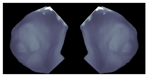
The streamlines can also be used to project a volume or xyz coordinates onto a flattened view of the dorsal cortex. The volume or points can be aggregated along the streamlines in different ways, e.g max, mean, median.

In this example we will project the Allen Atlas dwi volume onto the dorsal cortex projection. We will take the maximum value along the streamline for each voxel on the surface

from iblatlas.streamlines.utils import project_volume_onto_flatmap

ba = AllenAtlas(25)
proj, fig, ax = project_volume_onto_flatmap(ba.image, res_um=25, aggr='max', plot=True, cmap='bone')
ax.set_axis_off()

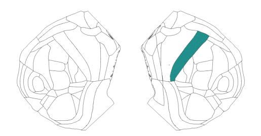
We can also do the same with xyz coordinates (we will use the same xyz coordinates for the region MOp and assign random values to each coordinate)

from iblatlas.streamlines.utils import project_points_onto_flatmap, get_mask

# Get a mask to plot our results on, options are 'image', 'annotation' or 'boundary
mask = get_mask('boundary')

values = np.random.rand(xyz.shape[0])

proj = project_points_onto_flatmap(xyz, values, aggr='mean', plot=False)
# Mask values with 0 with nan for display purposes
proj[proj == 0] = np.nan

fig, ax = plt.subplots()
ax.imshow(mask, cmap='Greys')
ax.imshow(proj)
ax.set_axis_off()